Using Customer-Specific Histories in Fraud Models

When it comes to the application of statistical models in the lending environment, the majority of the effort is dedicated to calculating the risk of bad debt; relatively little effort is dedicated to calculating the risk of fraud.

There are several good reasons for that, the primary one being that credit losses have a much larger impact on a lender’s profit.  Fraud losses tend to be restricted to certain situations and certain products: application fraud might affect many unsecured lending products but it does so to a lesser degree than total credit losses, while transactional fraud is typically restricted to card products.

I discuss application fraud in more detail in another article so in this one I will focus on modeling for transactional fraud and, in particular, how the assumptions underpinning these models vary from those underpinning traditional behavioural scoring models.

Credit Models

The purpose of most credit models is to forecast future behaviour.  Since the future of any particular account can’t be known, they do this by matching an account to a similar group of past accounts and making the assumption that this customer will behave in the same way as those customers did.  In other words, they ask the questions of each account, ’how much does this look like all previous known-bad accounts?’.

So if the only thing we know about a customer is that they are 25 years old and married, a credit model will typically look at the behaviour of all previous 25-year-old married customers and assume that this customer will behave in the same way going forward.

The more sophisticated the model, the more accurate the matching; and the more accurate the matching between the current and past customers, the more valid the transfer of the latter group’s future behaviour to the former will be.

Imagine the example below where numerical characteristics have been replaced with illustrative ones.  Here there are three customer groups: high risk, medium risk and low risk.  A typical low risk customer is blue with stars, while a high risk customer is red with circles and a medium risk customer is green with a diamonds.

A basic model would look at any new customer, in this case green with stars, and assign them to the group they  most closely matched – medium risk – and assume the associated outcome – a 3% bad rate.  A more sophisticated model would calculate the relative importance of the colour versus the shapes in predicting risk and would forecast an outcome somewhere between the medium and low risk outcomes.

An over-simplification but the concept holds well enough to suffice for this article.

The key difficulty a credit model has to overcome is that it needs to forecast an unknown future based on a limited amount of data.  This forces the model to group similar accounts and to treat them as the same.  To extend the metaphor from above, few low risk accounts would actually have been blue with stars; there would have been varying shades of blue and varying star-like shapes.  Yet it is impossible to model each account separately so they would have been grouped together using the best possible description of them as a whole.

Transactional fraud models need not be so tightly bound by this requirement, though the extra flexibility that this allows is often over-looked by analysts too set in the traditional ways.

Transactional Fraud Models

Many transactional fraud models take the credit approach and ask ’how much does this transaction look like a typical fraud transaction?’.  In other words, they start by separating all transactions into ‘fraud’ and ‘non fraud’ groups, identifying a ‘typical’ fraud transaction and then comparing each new transaction to that template.

However, rather than only asking the question ’how much does this look like a typical fraud transaction?’, a fraud model can also ask ’how much does this look like this cardholder’s typical transaction?’.

A transactional fraud model does not need to group customers or transactions together to get a view of the future, it simply needs to identify a transaction that does not meet a specific customer’s established spend pattern.  Assume a typical fraud case involves six transactions in a day, each of a value between €50 and €500 and with the majority of them occurring in electronic stores.  A credit-style model might create an alert whenever a card received its sixth transaction in a day totaling at least €300 or when it received its third transaction from an electronic store.  However, if it was known that the cardholder in question had not previously used their card more than twice in a single day and had never bought goods at any of the stores visited, that same alert might have been triggered earlier and been attached to a higher probability of fraud.

A large percentage of genuine spend on a credit cards is recurring; that is to say it happens at the same merchants month in and month out.  In a project on this subject, I found that an average of 50% of genuine transactions occurred at merchants that the cardholder had visited at least once in the previous six months (that number doesn’t drop much when one uses only the previous three months).  Some merchant categories are more susceptible to repeat purchases than others but this can be catered for during the modeling process.  For example you probably buy your groceries at one of three or four stores every week but you might frequently try a new restaurant.

The majority of high value fraud is removed from the customer by time and geography.  A card might be ’skimmed’ at a restaurant in London but that data might then be emailed to America or Asia where, a month later, it is converted into a new card to be used by a fraudster.  This means that fraudsters seldom know the genuine customer’s spend history and so matching their fraudulent spend to the established patterns is nearly impossible.  In the same project, over 95% of fraud occurred at merchants that the genuine cardholder had not visited in the previous six months.  Simply applying a binary cut-off based on whether the merchant in questions was a regular merchant would lead to a near doubling of hit rates from the existing rule set.

Maintaining Customer Histories

The standard approach to implementing a customer-specific history would be as illustrated above.  In the live environment new transactions are compared to the historical record and are flagged if the merchant is new or, in more sophisticated cases, if the transaction value exceeds merchant-level cut-offs.  The fact that this is outside of history is used as a prioritisation with other fraud rules to create alerts.  Then later, in a batch run, the history is updated with the data relating to new merchants and changes to merchant-level patterns.  If only a specific period worth of data is stored, then older data is dropped-off at this stage.  This is commonly done to improve response times with three to six months worth of data usually being enough.

Customer-specific patterns like this are not enough to indicate fraud but, when used in conjunction with an existing rule set in this way they can add significant value.

There are of course some downsides to this approach, primarily the amount of data that needs to be stored and accessed.  This is particularly true if your fraud rules are triggered during the authorisations process.  In these cases it may be necessary to sacrifice fraud risk for performance by using only basic rules in the authorizations system followed by the full rule set in the reactionary fraud detection system.  Most card issuers follow this sort of approach where the key goal of authorisations is good customer service through fast turn-around times rather than fraud prevention.

The amount of data stored and accessed should be matched to each issuer’s data processing capabilities.  As mentioned earlier, simply accessing a rolling list of previously visited merchants can double the hit rate of existing rules and is not a data-intensive process.  Including average values, GIS or other value-added data will surely improve the rule hit rates even further but will do so with added processing costs.

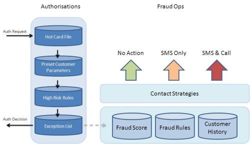
The typical implementation would look like the diagram below:

In this set-up, customer history is not queried live but is rather used to update a series of specific fields such as customer parameters and an exception file.  The customer parameters would be related to the value of spend typical to any one customer and could be updated daily or weekly – even monthly updates will be alright if sufficient leeway is included when these are calculated.  An exception file will include specific customers to whom the high risk fraud rules should not apply.  This is usually done to allow frequent high risk spenders or frequent users of high risk merchant types – often casinos – to spend without continuously hitting fraud rules.

Once an authorization decision has been made, that data is passed into the offline environment where it passes through a series of fraud rules and sometimes a fraud score.  It is in this environment that the most value can be attained from the addition of a customer-specific history.  Because this is an offline environment, there is more time to query larger data sets and to use that information to prioritise contact strategies which should always include the use of SMS alerts as described here.

Here the fact that a transaction has fallen outside of the historical norm will be used as an input into other rules.  For example, if there have been more than three transactions on an account in a day and at least two of those were at new merchants, a phone call is queued.

Read Full Post »

‘Cherry Picking’ Accounts in Collections

I wrote in my last article that a debt collection agency (DCA) working on a commission basis had the ability to ‘cherry pick’ the accounts that they worked, distributing their invested effort across multiple customer segments in multiple portfolios to generate significantly higher rewards.  In this article I will walk through a simple example of how a DCA could do this across three portfolios and then discuss how the same principles can be applied by primary lenders.

 

A DCA Example

A third-party DCA is collecting debts on behalf of three different clients, each of which pays the same commission rate and each of which has outsourced a portfolio of 60 000 debts. 

Half of the accounts in Portfolio A have a balance of €4 000 while the other half are split evenly between balances of €2 000 and balances of €5 500.  After running the accounts in question through a simple scorecard, the DCA was able to determine that 60% of the accounts are in the high risk group with only a 7% probability of payment, 20% are in the medium risk group with a 11% probability of payment while the remainder are in the low risk group and have a 20% probability of payment.

Portfolio B ia made-up primarily of account with higher balances, with half of the accounts carry a balance of €13 500 and the remainder are equally split between balances of €7 500 and €5 000.  Unfortunately, the risk of this portfolio is also higher and, after also putting this portfolio through the scorecard, the DCA was able to determine that 50% of the accounts were in the highest risk group with an associated probability of payment of just 2% while 30% of the accounts were in the medium risk group with a probability of payment of 5% and 20% of the accounts were in the lowest risk group with a probability of payment of 13%.

In portfolio C the accounts are evenly split across three balances: €4 500, €8 000 and €10 000.  After a similar scorecard exercise it was also shown that 70% of accounts are in the highest risk group with a 7.5% probability of payment, 30% of accounts are in the medium risk group with a probability of payment of 14% and the final 10% in the low risk group have an 18% probability of payment.

The DCA now has a few options when assigning work to its staff.  It could assign accounts randomly from across all three portfolios to the next available staff member, it could assign accounts from the highest balance to the lowest balance or it could assign specific portfolios to specific teams, prioritising work within each portfolio but not across them.  Some of these approaches are better than others but neither will deliver the optimal results.  To achieve optimal results, the DCA needs to break each portfolio into customer segments and then prioritise each of those segments; working the highest yielding segment first and the lowest yielding one last.

Using the balance and probability of payment information we have, it is possible to calculate a recovery yield for each of the nine segments in each portfolio; the recovery yield being simply the balance multiplied by the probability of recovering that balance.  Once the recovery yield has been determined for each of the nine segments in each of the three portfolios it is possible to prioritise them against each other as shown below.

With the order of priority determined, it is possible now to assign effort in the most lucrative way.  For example, if the DCA in question only had enough staff to work 50 000 accounts they would expect to collect balances of approximately €27.7 million if they worked the accounts randomly, approximately €40.4 million if they prioritised their effort based on balance but as much €53.3 million if they followed the recommended approach – an uplift of 92%.  As more staff become available so the less the apparent uplift decreases but there is still a 44% improvement in recoveries if 100 000 accounts can be worked.

If all accounts can be worked then, at least if we keep our assumptions simple, there is no uplift in recoveries to be gained by working the accounts in any particular order. 

 

Ideal Staff Numbers

However, that is not to say that the model becomes insignificant.  While the yield changes based on which segment an account is in, the cost of working each of those accounts remains the same.  Since profitability is the difference between yield and cost and since cost remains steady, a drop in yield is also a drop in profit.  So, continuing along that line of reasoning, there will be a level of yield below which a DCA is making a loss by collecting on an account.

So, it stands to reason then that a DCA working all accounts is unlikely to be making as much profit as they would be if they were to use the ‘cheery picking’ model to determine their staffing needs.  New staff should be added to the team for as long as they will add more value than they will cost.  As each new member of staff will be working on lower yield accounts there are diminishing marginal returns on staff until the point that a new member of staff will be actually value destroying.

Assume it costs €30 000 to employ and equip one collector and that that collector can work 1 500 accounts in a year.  To be value adding then, that collector must be assigned to work only accounts with a net yield of more than €20. 

Up to now, I simply referred to recovery yield as the total expected recovery from a segment.  That was possible at the time as we had made the simplifying assumption that each portfolio earned the same commission and were only looking to prioritise the accounts.  However, once we start to look at the DCA’s profit, we need to look at net yield – or the commission earned by the DCA from the recovery. 

If we assume a 10% commission is earned on all recoveries then for the yield of €1 800 in highest yielding segment becomes a net yield of €180.  Using that assumption we are able to see that the ideal staffing contingent for the example DCA is 104: allowing the DCA to work the 156 000 accounts in segment 24 and better. 

At this level the DCA will collect approximately €96 million earning themselves €9.6 million in commission and paying out €3.1 million in staff costs in the process; this would leave them with a profit of €6.4 million.  If they lay off two members of staff and work one less segment their profit would decrease by €6 000.  If, instead, they hired 5 more members of staff and worked one more segment their profits would be reduced by nearly €40 000.

Commission Rate Changes

Having just introduced the role of commission, it makes sense to consider how changes in commission rates might impact on what we have already discussed. 

The simplest change to consider is an across-the-board change in commission rates.  This doesn’t change the order in which accounts are worked as it affects all yields equally.  It does, however, change the optimal staff levels.  In the above example an across-the-board decrease in commission from 10% to 5% would halve the yields of each block meaning to still achieve a net yield of €20 a segment would have to have a gross yield of €400.  In turn this would mean that staff numbers would need to be cut back to 59: now working 88 000 accounts and generating a total profit of €2 million.

A more common scenario is that commissions are fixed over the term of the contract but that these commissions vary from portfolio to portfolio. 

Most DCAs will charge baseline commission rates which vary with the age of the debt at the time it is taken on.  For example, a DCA may charge a client 5% of all recoveries made on accounts handed over at 60 days in arrears but 10% of all recoveries made on accounts handed over at 120 days in arrears.  This compensates the DCA for the lower recovery rates expected on older debt and encourages primary lenders to outsource more debts to the DCA.

When a DCA is operating across portfolios which each earn different commission rates it should use the net yield in the prioritisation exercise described above rather than the gross yield.  Assume that the DCA from our earlier example actually earns a commission of 5% for all recoveries made from Portfolio A, 7.5% on all recoveries made from Portfolio B and 10% on all recoveries made from Portfolio C. 

Now, the higher rewards offered in Portfolio C change the order in which accounts should be worked.  The DCA no longer concentrates on the largest recovery yield but rather the largest net yield. 

Primary Lenders

Of course, the concept and models described here are not unique to the world of DCAs, primary lenders should structure their debt management efforts around similar concepts.  The only major difference during the earlier stages of the debt management cycle is that there tends to be more strategic options, more scenarios and a wider diversity of accounts.

This leads to a more complex model but one that ultimately aims to achieve the same end result: the optimal mix between cost and reward.  Again a scorecard forms the basis for the model and creates the customer segments mentioned above.  Again the size of the balance can be used as a proxy for the expected benefit.   There is of course no longer a commission but there are new complexities, including the need to cost multiple strategy paths and the need to calculate the recovery rate as the recovery rate of the strategy only – i.e. net of any recoveries that would have happened regardless.  For more on this you can read my articles on risk based collections and on self-cure models.

Read Full Post »

Risk Based Collections for Late-Stage Debt Collections

In the other articles I’ve written here I looked at risk-based collections strategies from a primary lender’s point-of-view and with a particular focus on the earlier stages of the process.  However, although the basic principles are universally applicable, there are a number of thought changes that need to be made when one is considering risk-based collections strategies from a third party’s point-of-view or when the debt in question has been delinquent for a longer period of time.  In this article I will try to highlight the most important of those changes.

 

Late Stage Collections

The most important difference between early stage collections and late stage collections is driven by changes to risk distribution over time.  A random group of accounts in early stage collections is likely to be made-up from a diverse distribution of actual account risks: a lot of low risk accounts, a lot of medium risk accounts, several high risk accounts and a few very high risk accounts.  As this group of accounts proceeds through the collections process the distribution becomes more homogeneous with a bias towards the more risky accounts.  This is not because there are more risky accounts present per se, but rather because most of the lower risk accounts have left collections.  As accounts proceed through collections it is the lower risk accounts that leave at a faster rate and the higher risk accounts therefore begin to dominate as illustrated below.

 

The practical implication of this is that it becomes harder and harder to segment accounts into risk groups.  Since risk-based strategies are built upon customer segmentation, it follows that these strategies also become more difficult to design.

For this reason, specialist scorecards and strategies are recommended for late stage collections.  In most cases, a traditional behavioural scorecard starts to lose its effectiveness as a debt portfolio reaches about 60 days of delinquency from where its performance drops steadily, seldom being of significant value after 120 days.

Early stage collections scorecards may add value for longer but once a debt has passed 210 days of delinquency a specialist scorecard is almost always needed.

Since the distribution of risk has been reversed, so too should be the focus of the scorecard.  Rather than trying to predict which few of the many good accounts will eventually go bad, the scorecard now needs to predict which few of the many bad accounts will eventually cure.  The traditional ‘bad definition’ is replaced with a ‘good definition’. 

The exact ‘good definition’ will vary with business requirements but is usually related to whether an account will make a payment, a certain number of consecutive payments or payments equal to a certain percentage of balance outstanding.

Specialised late stage collections scorecards of this kind tend to focus on events that happened post delinquency rather than pre-delinquency: number of times in collections, number of previous collection payments, promise-to-pays kept, number of negative bureau remarks, number of legal claims outstanding, etc. 

Despite their technical limitations, late stage scorecards can still offer significant value.  In a recent implementation of late stage scorecard built off very limited data I have seen a portfolio segmented and summarised into four risk groups with the 25% of accounts in the lowest risk group four times as likely to make a payment as the 25% of accounts in the highest risk group.

 

External Collections

Managing late stage collections is typically a drawn-out and operationally intensive processes.  For this reason, many lenders choose to outsource the function to third parties.

Once a debt has left the primary lender, its nature changes; most obviously because the ‘balance’ side of the lending profit model is no longer a consideration.  The third-party can no longer profit from commission or interest charges levied on new balance growth, can no longer charge annual fees and can no longer generate cross-sell opportunities.  So only the cost side of the traditional lending profit model remains. 

That is not to say that debt collection agencies don’t earn revenue of course, it’s just that they earn their revenue from the cost side of the traditional lending profit model; the side dealing with risk costs and bad debt losses.

There are two dominant business models for debt collection agencies based on whether the original debt was sold outright or merely outsourced by the primary lender.  When a debt collection agency buys a portfolio of debt outright, it tends to see that portfolio in a similar way to the primary lender.  When, on the other hand, it only collects the debts on the original lender’s behalf, the portfolio is usually viewed quite differently.

 

Purchased Debt

When a portfolio of debts is purchased by a debt collection agency they usually pay a price equal to a given percentage of the balances outstanding.  They then need to recover a high enough percentage of those balances to cover this initial price as well as all the operational costs that need to be incurred in making those recoveries.

This business model means that the buyer takes on all the risk inherent in a portfolio at the time of purchase and has little ability to adjust their level of investment thereafter.  The price paid at the start is the critical factor in overall profitability; managing the costs incurred in the collection process and using better techniques to gain an up-lift in recoveries usually make a lesser impact.

A debt collection agency interested in purchasing a new portfolio should therefore invest considerable time and resources to accurately estimate the expected recoveries from – and the expected cost of working – any new portfolio.

Unfortunately, these efforts are usually complicated by a lack of quality data.  It is uncommon for the purchaser to have access to extensive data relating to the portfolio for sale, often because this simply doesn’t exist but also sometimes due to a reluctance to share data on the part of the seller.  Therefore, it is often necessary to make some compromises.

The best way to deal with a lack of specific data is to deploy a generic model.  Generic models can either be built in-house (if the purchaser has experience collecting debts on other, similar portfolios) or they can be purchased from a specialist firm with access to pooled industry data. 

Rather than running accounts through the generic scorecard on a case-by-case basis as one would if it were deployed in its typical form, the scorecard is used to segment a random sample of accounts from the new portfolio in order to create an estimate of that portfolio’s total risk make-up.  The expected recovery rates of the model create a baseline estimate for the expected recovery rate of the portfolio.  The generic strategy paths of the model can be used to create a baseline estimate for the cost of the recovery.

This baseline can then be adjusted upwards or downwards to take into account any variance from the norm the purchaser expects to stem from their own environment: for example the expected recover rate would be adjusted downwards if the purchaser had never collected a debt in the market in question or upwards if they had a track record of consistently achieving higher than average recoveries.

A generic scorecard might be less accurate than a bespoke scorecard would be in each specific case but it is more broadly applicable than the bespoke scorecard would have been.  A generic approach is also quicker and cheaper to implement.  This will be the preferable solution, therefore, whenever there is either simply no data with which to build a bespoke model or where the total value of the portfolio does not justify a larger investment.

 

Third-Party Debt

If the debt collection agency has not bought the portfolio outright but is collecting on behalf the primary lender or debt owner, the profit model changes somewhat.  Unlike the traditional lending model, the profit model of the third-party debt collector is not heavily influenced by bad debt write-offs.  Instead of incurring small risk costs for each account in arrears and large write-off costs, the third-party debt collector earns a fee or commission for every recovery made.  This means that if a large debt is written-off there is no direct cost as such, just a lost opportunity for a commission-earning recovery. 

Since the commission is usually a small percentage of the total balance outstanding the impact of balance size is diluted; but the cost to make a recovery is relatively unchanged so the focus shifts to ‘cherry picking’.  For a given operational cost it can be more profitable to contact the accounts that are most likely to pay than it is to try to prevent large balance accounts that are at risk of defaulting from doing so.

Using a combination of the expected recovery rate and the expected recovery value on a recent project, we were able to identify segments of a portfolio that generated returns over 8 times higher than the average returns for that portfolio.  Identifying and focusing on similar segments from each of its portfolios, rather than treating each portfolio as internally and externally homogenous, will allow a debt collection agency to generate significantly higher profits by ensuring all high yield opportunities are followed while all low yield opportunities are not pursued.

This ability to shift effort to where it is most profitable is the key difference between the two business models.  While the eventual profitability of a single deal is still dominated by the contracted commission rates, the debt collection agency can more easily shift their investment to other more profitable deals as soon as it becomes apparent that the actual recovery rates on a given portfolio are lower than initially expected. 

Assume a debt collection agency has signed a new contract to collect debt on a lender’s behalf in return for a commission of 10% of all recoveries.  Assume too that they signed the deal at this price because their internal calculations suggested that they would receive payments from every second debtor which, in turn, would be sufficient to cover their costs and profit requirements.  If, after a month of working the new portfolio, that they were to discover that they were only receiving payments from every fourth debtor they could reduce the number of staff they had working on the new portfolio and re-assign them to more profitable work on another portfolio; restricting their efforts on the new portfolio to only those customer segments identified as still profitable.

In reality, contracts signed between lenders and agencies try to overcome this problem so the application of the theory is seldom this ‘clean’.  In most cases a large primary lender will assign their debt to more than one collections agency to allow a comparison of the performance of each against the other.  They usually then distribute their debt in a ratio based on that performance so that, for example, the best performing agency may receive 60% of all outsourced debt, the second best agency 30% and the worst agency 10%. 

Clauses like this complicate the calculation of optimal investments but don’t change the fact that it is still possible for a third-party debt collector to adjust their level of investment in any one portfolio as more information is learned.

*   *   *   *   *

I have been asked before how a debt collection agency can optimise the timing of when they hand accounts over to lawyers.  The model I suggest for these cases is an adaptation of the self-cure model I introduced in a previous article.  Rather than dedicate a whole article to this version, I have included a discussion here.  However, since the subject matter is a bit more technical from here onwards it may be of less interest to some readers.

 

Escalating to Legal

Once an account has reached an external debt collection agency there are not many options left in terms of further escalation; if an account leaves a debt collection agency it can either move sideways to another debt collection agency, be written-off or escalated to legal recoveries.

Knowing which of these routes is best for each account is an important factor in determining the overall profitability of a third-party debt collector.  The approach I would recommend is the same one I discussed here when talking about self-cure models.

It is the nature of the debt collection business that much of the work will go unrewarded, with only a small portion of accounts generating meaningful payments.  It is important to not over-invest in accounts where the likelihood of recoveries is too low.  However, since all accounts have already demonstrated either a lack of willingness to pay or a lack of ability to pay, determining when the likelihood to recover is too low is easier said than done.

The factors involved are very similar to those at play in a self-cure model where one is also seeking to not over-invest in accounts while simultaneously not compromising the long-term recovery rate of the portfolio by not working an account that may consequently go bad where they might otherwise not have.  In the case of a self-cure model the goal is to avoid needlessly paying to contact debtors that will pay regardless of a contact and in the case of an escalation model the table has been turned so the goal is to avoid needlessly paying to contact a debtor that will not pay regardless of a contact.

In order to calculate the optimal time to change the treatment of an account it is important to know the direct costs and expected benefits of each strategy and, most importantly, how those change over time. 

The expected recovery from a telephone and letter based debt collection strategy decreases over time.  Once a delinquent customer has been contacted telephonically on multiple occasions the probability of the next contact making a difference is small.  The expected recovery from a legal recovery strategy decreases more slowly.  The cost of each method is also different, with the standard approach having a small but regular cost where the legal method usually has a high but largely fixed cost associated.  It is these differences that create an opportunity to profit from a change in strategy.

In summary, the cheaper method should always be employed unless the lost opportunity for recoveries from not using the more expensive method outweighs those savings.  So, in the case of a debt collection agency an account should be retained for the next period unless the decrease in expected recoveries from a legal recoveries strategy over the same period is greater than the cost difference between the two methods as shown in the table below.

 

Name(required)

Email(required)

Website

Comment(required)

Submit

Δ

Read Full Post »

A Generic Credit Card Profit Model

*** This article is being moved to my new website, you can click here to be redirected to the latest version: https://www.howtolendmoneytostrangers.show/articles/what-does-a-lender-look-like-on-the-inside

If you’re interested in this content, you may also be interested in the podcast I’ve started there, too: https://www.howtolendmoneytostrangers.show/episodes

Probably the most common credit card business model is for customers to be charged a small annual fee in return for which they are able to make purchases using their card and to only pay for those purchases after some interest-free period – often up to 55 days.  At the end of this period, the customer can choose to pay the full amount outstanding (transactors) in which case no interest accrues or to pay down only a portion of the amount outstanding (revolvers) in which case interest charges do accrue.  Rather than charging its customer a usage fee, the card issuer also earns a secondary revenue stream by charging merchants a small commission on all purchases made in their stores by the issuer’s customers.

So, although credit cards are similar to other unsecured lending products in many ways, there enough important differences that are not catered for in the generic profit model for banks (described here and drawn here) to warrant an article specifically focusing on the credit card profit model.  Note: In this article I will only look at the profit model from an issuer’s point of view, not from an acquirer’s.

* * *

We started the banking profit model by saying that profit was equal to total revenue less bad debts, less capital holding costs and less fixed costs.  This remains largely true.  What changes is the way in which we arrive at the total revenue, the way in which we calculate the cost of interest and the addition of a two new costs – loyalty programmes and fraud.  Although in reality there may also be some small changes to the calculation of bad debts and to fixed costs, for the sake of simplicity, I am going to assume that these are calculated in the same way as in the previous models.

 

Revenue

Unlike a traditional lender, a card issuer has the potential to earn revenue from two sources: interest from customers and commission from merchants.  The profit model must therefore be adjusted to cater for each of these revenue streams as well as annual fees.

Total Revenue  = Fees + Interest Revenue + Commission Revenue

= Fees + (Revolving Balances x Interest Margin x Repayment Rate) + (Total Spend x Commission)

= (AF x CH) + (T x ATV) x ((RR x PR x i) + CR)

Where              AF = Annual Fee                                               CH = Number of Card Holders

T = Number of Transactions                          PR = Repayment Rate

ATV = Average Transaction Value              i = Interest Rate

RR = Revolve Rate                                              CR = Commission Rate

Customers usually fall into one of two groups and so revenue strategies tend to conform to these same splits.  Revolvers are usually the more profitable of the two groups as they can generate revenue in both streams.  However, as balances increase and approach the limit the capacity to continue spending decreases.  Transactors, on the other hand, seldom carry a balance on which an issuer can earn interest but they have more freedom to spend.

Strategies aimed at each group should be carefully considered.  Balance transfers – or campaigns which encourage large, once-off purchases – create revolving balances and sometimes a large, once-off commission while generating little on-going commission income.  Strategies that encourage frequent usage don’t usually lead to increased revolving balances but do have a more consistent – and often growing – long-term impact on commission revenue..

Variable Costs

There is also a significant difference between how card issuers and other lenders accrue variable costs.

Firstly, unlike other loans, most credit cards have an interest free period during which the card issuer must cover the costs of the carrying the debt.

The high interest margin charged by card issuers aims to compensate them for this cost but it is important to model it separately as not all customers end up revolving and hence, not all customers pay that interest at a later stage.  In these cases, it is important for an issuer to understand whether the commission earnings alone are sufficient to compensate for these interest costs.

Secondly, most card issuers accrue costs for a customer loyalty programme.  It is common for card issuers to provide their customers with rewards for each Euro of spend they put on their cards.  The rate at which these rewards accrue varies by card issuer but is commonly related in some way to the commission that the issuer earns.  It is therefore possible to account for this by simply using a net commission rate.  However, since loyalty programmes are an important tool in many markets I prefer to keep it out as a specific profit lever.

Finally, credit card issuers also run the risk of incurring transactional fraud –  lost, stolen or counterfeited cards.  There are many cases in which the card issuer will need to carry the cost of fraudulent spend that has occurred on their cards.  This is not a cost common to other lenders, at least not after the application stage.

Variable Costs = (T x ATV) x ((CoC x IFP) + L + FR)

Where            T = Number of Transactions                         IFP = Interest Free Period Adjustment

ATV = Average Transaction Value             CoC = Cost of Capital

FR = Fraud Rate

Shorter interest free periods and cheaper loyalty programmes will result in lower costs but will also likely result in lower response rates to marketing efforts, lower card usage and higher attrition among existing customers.

 

The Credit Card Profit Model                   

Profit is simply what is left of revenue once all costs have been paid; in this case after variable costs, bad debt costs, capital holding costs and fixed costs have been paid.

I have decided to model revenue and variable costs as functions of total spend while modelling bad debt and capital costs as a function of total balances and total limits.

The difference between the two arises from the interaction of the interest free period and the revolve rate over time.  When a customer first uses their card their spend increases and so does the commission earned and loyalty fees and interest costs accrued by the card issuer.  Once the interest free period ends and the payment falls due, some customers (transactors) will pay their full balance outstanding and thus have a zero balance while others will pay the minimum due (revolve) and thus create a balance equal to 100% less the minimum repayment percentage of that spend.

Over time, total spend increase in both customer groups but balances only increase among the group of customers that are revolving.  It is these longer-term balances on which capital costs accrue and which are ultimately at risk of being written-off.  In reality, the interaction between spend and risk is not this ‘clean’ but this captures the essence of the situation.

Profit = Revenue – Variable Costs – Bad Debt – Capital Holding Costs – Fixed Costs

= (AF x CH) + (T x ATV) x ((RR x PR x i) + CR) – (T x ATV) x (L + (CoC x IFP)) – (TL x U x BR) – (TL x U x CoC +   TL x   (1 – U) x BHR x CoC) – FC

= (T x ATV) x (CR – L – (CoC x IFP) -FR) – (TL x U x BR) – ((TL x U x CoC) + (TL x (1 – U) x BHR x CoC)) – FC

Where        AF = Annual Fee                                               CH = Number of Card Holders

T = Number of Transactions                         i = Interest Rate

ATV = Average Transaction Value               TL = Total Limits

RR = Revolve Rate                                                U = Av. Utilisation

PR = Repayment Rate                                          BR = Bad Rate

CR = Commission Rate                                        CoC = Cost of Capital

L = Loyalty Programme Costs                          BHR = Basel Holding Rate

IFP = Interest Free Period Adjustment        FC = Fixed Costs

FR = Fraud Rate

 

Visualising the Credit Card Profit Model  

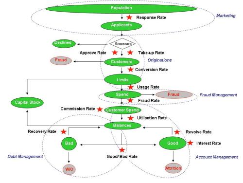
Like with the banking profit model, it is also possible to create a visual profit model.  This model communicates the links between key ratios and teams in a user-friendly manner but does so at the cost of lost accuracy.

The key marketing and originations ratios remain unchanged but the model starts to diverge from the banking one when spend and balances are considered in the account management and fraud management stages.

The first new ratio is the ‘usage rate’ which is similar to a ‘utilisation rate’ except that it looks at monthly spend rather than at carried balances.  This is done to capture information for transactors who may have a zero balance – and thus a zero balance – at each month end but who may nonetheless have been restricted by their limit at some stage during the month.

The next new ratio is the ‘fraud rate’.  The structure and work of a fraud function is often similar in design to that of a debt management team with analytical, strategic and operational roles.  I have simplified it here to a simple ratio of fraud: good spend as this is the most important from a business point-of-view, however if you are interested in more detail about the fraud function you can read this article or search in this category for others.

The third new ratio is the ‘commission rate’.  The commission rate earned by an issuer will vary by each merchant type and, even within merchant types, in many cases on a case-by-case basis depending on the relative power of each merchant.  Certain card brands will also attract different commission rates; usually coinciding with their various strategies.  So American Express and Diners Club who aim to attract wealthier transactors will charge higher commission rates to compensate for their lower revolve rates while Visa and MasterCard will charge lower rates but appeal to a broader target market more likely to revolve.

The final new ratio is the revolve rate which I have mentioned above.  This refers to the percentage of customers who pay the minimum balance – or less than their full balance – every month.  On these customers an issuer can earn both commission and interest but must also carry higher risk.  The ideal revolve rate will vary by market and depending on the issuers business objectives but should be higher when the issuer is aiming to build balances and lower when the issuer is looking to reduce risk.

Name(required)

Email(required)

Website

Comment(required)

Submit

Δ

Read Full Post »

Building a Self-Cure Strategy in Collections

The Space Pen

We’ve surely all heard the old story of how, during the space race, America invested millions of dollars to develop a pen that could write in the zero gravity conditions of space while the Russian achieved the same goal using the humble pencil.  Over the years much of the story has been exaggerated for the sake of its telling but its key lesson has remained the same: where there are two ways of achieving a goal, the cheapest of these methods is best. 

In this story the goal was to allow astronauts to write without gravity driving the flow of ink flow through a traditional pen.  It could have been achieved using an expensive pen with pressurised ink or, so the story implies, just as easily using a cheap pencil.

Learnings for Debt Management

If we were to apply the learnings to our debt management function, doing so would surely back-up the case for implementing a broadly inclusive self-cure strategy: that is a strategy that allows debtors a period of time in which to pro-actively repay their outstanding debt before investing the organisation’s time and money to contact them re-actively to make a direct request for that payment.  Since the value of a collections recovery is the same regardless of how it is achieved, it makes sense that the method used to generate that recovery should be the cheapest effective method available.  And, likewise, it makes sense that the cheapest method would be the one in which no costs are incurred.

However, by delving deeper into the history of the space pen we find that some caution is required before making that logical leap.

You see, the real story behind the space pen does not end at the same point that the anecdote does.  In fact, there are two pertinent points that are seldom mentioned.  Firstly, NASA had been using pencils prior to the development of the space pen and had decided they needed to be replaced.  Secondly, after the introduction of space pens at NASA, the Russians also started to use them.

Why would both teams have replaced the cheaper solution with a more expensive one if both did the same job?  Well it turns out that they had identified several indirect costs of pencil use; broken pieces of pencil lead can pose a risk in a zero gravity environment and the wood is flammable.

So the key lesson of the story remains true: the cheapest affective method to solve a given problem is the best method.  However, the measurement of ‘cheapest’ must include all direct and indirect costs.  This is true as much for a debt management function as it is for the space programme.

When designing a comprehensive self-cure strategy therefore, a lender must understand both is expected benefits and its direct and indirect costs before deciding who to include and for how long.

Estimating the Expected Benefits of a Self-Cure Strategy

The expected benefit of a self-cure strategy is simply the expected number of payment agreements to be achieved as a percentage of all customers in the strategy – or the probability or payment. 

A standard risk based collections strategy will segment customers into a number of risk groups each of which can then be treated differently.  As a natural product of this, each of these groups will have a known probability of payment based on their observed behaviour over time.  But it is important to take care when using these numbers in relation to a proposed self-cure strategy.

The probabilities of payment associated with the existing risk groups inherently assume that each account will proceed through the current debt management operational strategies as before.  By making that assumption invalid, you make the numbers invalid.  The expected benefit of a self-cure strategy can therefore not be assumed to be equal to the currently observed probability of payment; they actual probabilities of payment will likely be significantly lower.

Therefore, early iterations of a self-cure strategy should include a number of test-and-learn experiments designed to determine the probability of payment under a self-cure strategy.  A good starting point is to allow a test group a very short self-cure period – perhaps just two or three days.  In many organisations this amounts to little more than de-prioritising these accounts so that the time taken to work through the rest of the accounts can serve as the self-cure period.  Once the basic risk assumptions have been tested, the self-cure period can be extended – though usually to not longer than fifteen days.

It is also important to note that the probability of payment must not be measured as a single, static figure.  The way it will be applied in the eventual self-cure model means that it is important to measure how the probability of payment changes over time.

Some customers in the early stages of debt management will be ‘lazy payers’, that is customers who have the will and means to meet their obligations but tend to pay late on a regular basis; their payments will likely come in the first few days after the due date.  Other customers may have been without access to their normal banking channels for whatever reason; their payments may be more widely spread across the days after due date.  Regardless of the exact reasons, in most portfolios the majority of self-cure payments will come in the first few days after due date and thereafter at an ever-slowing rate.

Estimating the Costs of a Self-Cure Strategy

If there were direct costs involved in a self-cure model, there would be a break-even point where the dropping effectiveness and the ongoing costs of the strategy would make it inefficient to continue.  However, because a self-cure strategy has no such direct costs the problem needs to be looked at differently.

But, as I mentioned earlier, a valuable lesson can be learned by following the story of the space pen all the way to its real conclusion: the total cost of a solution is never its direct costs alone but also includes all of its indirect costs.  In the space race, the pencil’s low direct cost was nullified by its high indirect risk costs.  In debt management, a self-cure strategy’s low direct cost may also be nullified by its high indirect risk costs.

The indirect risk costs of a self-cure strategy stem from the fact that the probability of making a recovery decreases as the time to make a customer contact increases.  Customers who are in arrears with one lender are likely to also have other pressing financial obligations.  While the one lender may follow a self-cure strategy and hold off on a direct request for repayment, their debtor may re-prioritise their funds and pay another, more aggressive, lender instead. So, while waiting for a free self-cure payment to come in a lender is also reducing their chances of making a recovery from the next best method should it become clear at a point in the future that no such payment is likely to be forthcoming. 

The cost of a self-cure strategy is therefore based on the rate at which the probability of receiving a payment from next best strategy decreases.  For every day that a self-cure strategy is in force the next best strategy must start one day later and this is the key cost to bear in mind.  Is one week of potential cheap recoveries from the self-cure model worth one week of opportunities lost for more expensive but more certain recoveries in the phone base collection strategy?

Building a Self-Cure Strategy

A self-cure strategy should be applied to all accounts for as long as they remain sufficiently likely to make a payment to compensate for the indirect costs of the self-cure strategy incurred by foregoing the opportunity to drive payments using the next best strategy.

As stated, the benefits of the strategy are equal to the probability of payment over a period of time and the costs are equal to the decrease in the probability of payment from the next best strategy over that same period.

If a customer is as likely to make a payment when they are called on day one as they are when called on day five, then there is no cost in a self-cure strategy for those first five days.  Therefore, no call should be made until day six regardless of how small the probability of receiving a payment from the self-cure strategy actually is.  This is because, with no costs, any recovery made is value generating and any recovery not made is value neutral. 

However, if after the first five days a customer who has not been contacted begins to become less likely to make a payment when eventually called, costs start to accrue.  The customer should remain in the self-cure strategy up to the point where the probability of payment from the self-cure strategy is expected to drop to a level lower than the associated drop in the probability of payment from the next best strategy.

The ideal time to move an account out of the self-cure strategy and into the next best strategy would be at the end of the period preceding the one in which this cross over of cost and benefit occurs.

Please note that the next best strategy does actually have a direct cost.  Strictly speaking, this direct cost should be added to the benefit of the self-cure strategy at each point in time.  However, in the early collections stages the next best strategy is usually cheap (text messages, letters or phone calls, etc.) and so these costs are insignificant.  However, if the next best strategy is expensive – legal collections or outsourcing for example – these costs could become a material consideration.  For the sake of simplicity I will not include the direct cost of the next best strategy in this discussion but will in an upcoming article covering the question of when to sell a bad debt/ escalate it to legal.

Summary

The cheapest method should always be used to make a recovery in debt management but, before the cheapest method can be identified, all direct and indirect cost must be understood.

I haven’t set out to discuss all the direct and indirect costs of debt management strategies here – not even all the direct and indirect costs of self-cure strategies.  Rather, I have attempted to explain the most important indirect costs involved in self-cure strategies and how it can be used to identify the ideal point at which an account should be moved out of a self-cure strategy and into the first lender-driven debt management strategy.

This point will vary based on each customer’s risk profile and the effectiveness of existing debt management strategies.  The probability of payment for the next best strategy will decrease faster for higher risk customers than for lower risk customers; bringing forward the ideal point of escalation.  The probability of payment will fall slower for more intense collection techniques (such as legal collections) than for soft collections techniques (such as SMS) but costs also vary; the structure of an organisation’s debt management function will also move the ideal point of escalation.

Finally, you might find it strange that I didn’t talk about which clients should be included in a self-cure strategy.  The reason is that, in theory, every customer should first be considered for a self-cure strategy.  The important part of this statement is that I used the words ‘considered for’ not ‘included in’.  Because of the mechanics of the model proposed, higher risk customers may well have an ideal point of escalation that is equal to the day they enter debt management and so, while ‘considered’ for inclusion in the self-cure strategy they won’t actually be ‘included’.  At the same time, medium risk customers may be included and escalated after five days while the lowest risk customers may be included and escalated only on the fifteenth day.  This will all vary with your portfolio’s make-up and so it is equally possible that no customer group will be worth leaving in a self-cure strategy for more than a day or two.

Read Full Post »